Author Archives: Jared Moore

Changing X-Axis Ticks in Holoviews Categorical Axis

I recently ran into the issue of changing how many ticks I want displayed on the x-axis in a holoviews plot. My data ranged from 0 to 100, but it was categorical in the pandas dataframe. Simple solutions don’t work in this case as categorical data can’t have the ticks changed easily in opts. Instead, I found this solution at: https://stackoverflow.com/questions/49460699/bokeh-plot-custom-categorical-tick-labels

Implementing it in my case allowed me to go from:

Far too many ticks on the x-axis to be readable. Importance is just noting that the objectives increase from left to right and not so much each individual one.

To this:

Much cleaner presentation by removing the extra information on the x-axis.

Code for the solution is below. Mainly, making the CategoricalAxis not visible and adding in a LinearAxis with FixedTicker did the trick.

import holoviews as hv

from bokeh.models import CategoricalTicker, FixedTicker, Ticker
from bokeh.models.formatters import NumeralTickFormatter
from bokeh.util.compiler import TypeScript
from bokeh.plotting import show
from bokeh.io import output_notebook, export_png
from bokeh.models.axes import LinearAxis
from bokeh.layouts import gridplot
    
def format_x_axis(p):
    # Remove default axis
    p.xaxis.visible = False

    # Add custom axis
    ticker = FixedTicker(ticks=[0,50,100])
    xaxis = LinearAxis(ticker=ticker)
    xaxis.axis_label = "Objective"
    p.add_layout(xaxis, 'below')
    
    return p

# Create a box plot to show how turning performs
def create_boxwhisker_custom_ticks(df, group_col, y_col, title, ylim=(-1.2,0)):
    boxwhisker = hv.BoxWhisker(df, [group_col], y_col).opts(width=300,xrotation = 90,ylim=ylim, title=title)
    return boxwhisker

plots = []
plot_width = 400
plot_height= 200

for t in wt_treatments:
    t += "_wt"
    filtered_df = wt_best_last_gen_per_rep_full_results_df[wt_best_last_gen_per_rep_full_results_df.Trt == t]
    filtered_df = filtered_df[filtered_df.Task == "wall"]
    wall = create_boxwhisker_custom_ticks(filtered_df, 'Subtask', 'Fitness', f'{wt_treatment_mapping[t]} Wall Crossing').opts(width=plot_width, height=plot_height)
    wall = format_x_axis(hv.render(wall))
    
    filtered_df = wt_best_last_gen_per_rep_full_results_df[wt_best_last_gen_per_rep_full_results_df.Trt == t]
    filtered_df = filtered_df[filtered_df.Task == "turn"]
    turn = create_boxwhisker_custom_ticks(filtered_df, 'Subtask', 'Fitness', f'{wt_treatment_mapping[t]} Turning').opts(width=plot_width, height=plot_height)
    turn = format_x_axis(hv.render(turn))
    
    plots.append([wall,turn])

# make a grid
grid = gridplot(plots)
show(grid)    

Holoviews: Sort Categorical Axis

One of the challenges when working with categorical data in pandas and Holoviews can be ordering appearance in a plot. To get around this, if you sort the pandas dataframe prior to sending the data to your Holoviews boxplot you can avoid the issue.

Source for example: https://stackoverflow.com/a/63508053

# Sort the df by Treatment for later ordering.
def trt_sorter(column):
"""Sort function"""
trt_order = ['1_naive','2_naive_wc','2_even-shuf_wc','2_flip1_wc','2_flip50_wc']
correspondence = {trt: order for order, trt in enumerate(trt_order)}
return column.map(correspondence)
Remove the "10000" from treatments.
df['Treatment'] = df['Treatment'].map(lambda x: x.rstrip('_10000'))
df = df.sort_values(by="Treatment", key=trt_sorter)

Bokeh or Holoviews and Chromedriver not found.

chromedriver becomes an impediment to generating png files from Bokeh and Holoviews.  It seems that chromedriver and Chrome are tied in terms of versions, so in between working on visualization projects Chrome updates and the old chromedriver doesn’t work.  This requires downloading a new chromedriver based on the currently installed Chrome version from https://chromedriver.chromium.org/getting-started.

Once there, move the downloaded chromedriver that matches your Chrome version into a folder on your path.  “/usr/local/bin” is one possible location.  Then approve the security settings when trying to run it the first time and you should be good to generate plots going forward.

A pesky issue that crops up, but not too bad if you write a blog post to remind future self what you just spent 20 minutes troubleshooting 🙂  (Or write a blog post after the third time you’ve had to figure out how to do this again!)

A handy code snipped to test chromedriver outside of working with a plot:

from selenium import webdriver

driver = webdriver.Chrome() # Optional argument, if not specified will search path.

driver.get('http://www.google.com/');

Of course, this code presupposes you placed chromedriver in a folder on your system PATH.

Bokeh Boxplot Color by Factor and Legend Outside Plot

The current version of Bokeh 0.12.10 broke some previous functionality for boxplots and required building a boxplot from the ground up. Unfortunately, the example code provided in the user guide colors each box based on the upper and lower boxes, rather than by the factor value. This example code instead colors by factor, and places the legend outside the bounding box. Full source code of this notebook is provided at: Bokeh Notebook Example.

First, we import the required packages, primarily pandas and bokeh.

import pandas as pd
import random

from bokeh.io import output_notebook
from bokeh.plotting import figure, output_file, show
from bokeh.models import ColumnDataSource

Next, we create some sample data. Not the most interesting, but formatting by factor and value allows us to create the boxplot.

# Generate some synthetic data.
df = pd.DataFrame({
    'Treatment':[str(i) for i in range(4) for j in range(100)],
    'y':[random.gauss(i, 0.5) for i in range(4) for j in range(100)]
})
df.head()

Now that we have some data, we first need a way to figure out how many colors we need. I wrote this convenience function to look at the data frame and figure out how many unique values are in the given column. Thus, we are coloring based on that column and pulling from the Spectral template built into bokeh.palettes. This function was adapted from the links provided in the code comments.

from bokeh.palettes import brewer
def color_list_generator(df, treatment_col):
    """ Create a list of colors per treatment given a dataframe and 
        column representing the treatments.
        
        Args:
            df - dataframe to get data from
            treatment_col - column to use to get unique treatments.
                
        Inspired by creating colors for each treatment 
        Rough Source: http://bokeh.pydata.org/en/latest/docs/gallery/brewer.html#gallery-brewer
        Fine Tune Source: http://bokeh.pydata.org/en/latest/docs/gallery/iris.html
    """
    # Get the number of colors we'll need for the plot.
    colors = brewer["Spectral"][len(df[treatment_col].unique())]

    # Create a map between treatment and color.
    colormap = {i: colors[k] for k,i in enumerate(df[treatment_col].unique())}

    # Return a list of colors for each value that we will be looking at.
    return [colormap[x] for x in df[treatment_col]]

The full code for the boxplot creating is below. We first get the colors needed for the treatments, four in our case. Next, get the categories we will be plotting by. Quartiles and interquartile range are then calculated. ‘upper_source’ and ‘lower_source’ are ‘ColumnDataSource’ objects needed to create the upper and lower quartile boxes for the boxplot. They are essentially dictionaries but with additional features documented in Bokeh. Here we specify not only the treatment values, but also the colors that we will fill each box by. Outliers are then identified and kept in their own data source.

The key insight of the Bokeh process is that the boxplot is built up by components, whiskers, vertical lines and boxes. Each of these calls is made using ‘segment’, ‘vbar’, and ‘rect’ calls. However, even though we have multiple treatments, by using the ‘ColumnDataSource’ objects, we are able to make one call to create a geom object for each treatment.

Finally, placing the legend outside the plot requires a bit of wrangling. This new feature in more recent versions of Bokeh is not well documented. We must build the legend ourselves and then place it manually. This can be done in two lines of code. The first creates the ‘Legend’ object by using the ‘vbar’ return renderer saved in the ‘l’ variable. Combining this with the ‘ColumnDataSource’ provided to the original renderer, we create the legend with four values, each corresponding to a treatment. Finally, we add the legend to the plot manually.

# Generate a boxplot of the maximum fitness value per treatment.
import numpy as np

from bokeh.models import Legend, LegendItem
from bokeh.plotting import figure, show, output_file

output_notebook()

# Get the colors for the boxes.
colors = color_list_generator(df, 'Treatment')
colors = list(set(colors))

# Get the categories that we will be plotting by.
cats = df.Treatment.unique()

# find the quartiles and IQR for each category
groups = df.groupby('Treatment')
q1 = groups.quantile(q=0.25)
q2 = groups.quantile(q=0.5)
q3 = groups.quantile(q=0.75)
iqr = q3 - q1
upper = q3 + 1.5*iqr
lower = q1 - 1.5*iqr

# Form the source data to call vbar for upper and lower
# boxes to be formed later.
upper_source = ColumnDataSource(data=dict(
    x=cats, 
    bottom=q2.y,
    top=q3.y,
    fill_color=colors,
    legend=cats
))

lower_source = ColumnDataSource(data=dict(
    x=cats, 
    bottom=q1.y,
    top=q2.y,
    fill_color=colors
))

# find the outliers for each category
def outliers(group):
    cat = group.name
    return group[(group.y > upper.loc[cat]['y']) | (group.y < lower.loc[cat]['y'])]['y']
out = groups.apply(outliers).dropna()

# prepare outlier data for plotting, we need coordinates for every outlier.
if not out.empty:
    outx = []
    outy = []
    for cat in cats:
        # only add outliers if they exist
        if not out.loc[cat].empty:
            for value in out[cat]:
                outx.append(cat)
                outy.append(value)

p = figure(tools="save", title="", x_range=df.Treatment.unique())

# stems (Don't need colors of treatment)
p.segment(cats, upper.y, cats, q3.y, line_color="black")
p.segment(cats, lower.y, cats, q1.y, line_color="black")

# Add the upper and lower quartiles
l=p.vbar(source = upper_source, x='x', width=0.7, bottom='bottom', top='top', fill_color='fill_color', line_color="black")
p.vbar(source = lower_source, x='x', width=0.7, bottom='bottom', top='top', fill_color='fill_color', line_color="black")

# whiskers (almost-0 height rects simpler than segments)
p.rect(cats, lower.y, 0.2, 0.01, line_color="black")
p.rect(cats, upper.y, 0.2, 0.01, line_color="black")

# outliers
if not out.empty:
    p.circle(outx, outy, size=6, color="#F38630", fill_alpha=0.6)

# Using the newer autogrouped syntax.
# Grab a renderer, in this case upper quartile and then
# create the legend explicitly.  
# Guidance from: https://groups.google.com/a/continuum.io/forum/#!msg/bokeh/uEliQlgj390/Jyhsc5HqAAAJ
legend = Legend(items=[LegendItem(label=dict(field="x"), renderers=[l])])

p.add_layout(legend, 'below')    

# Setup plot titles and such.
p.title.text = "Boxplot with Colored Treatments and Legend Outside Plot"
p.xgrid.grid_line_color = None
p.ygrid.grid_line_color = "white"
p.grid.grid_line_width = 2
p.xaxis.major_label_text_font_size="0pt"
p.xaxis.major_label_orientation = np.pi/4
p.xaxis.axis_label="Treatment"
p.yaxis.axis_label="y"
p.legend.location = (100,10)

show(p)

The final result should look something like this:

bokeh_plot

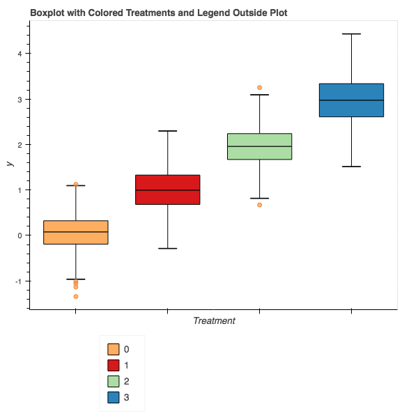
While perhaps not the most straightforward process compared to other plotting packages, Bokeh gives us the ability to build plots optimized for the web and additional features over just a static object. This code can of course be wrapped in a function and made part of a library, but that will be upcoming.

Color Points by Factor with Bokeh

Bokeh (https://bokeh.pydata.org/en/latest/) has been on my radar for some time as I move my data processing primarily to Jupyter notebooks.  The look and feel of the plots have sensible defaults and generally are visually pleasing without too much customization.  Compared to matplotlib, I find that I need to do much less customization to get my final product.

Unfortunately, sometimes the process of generating a plot isn’t a one-to-one mapping with my prior experiences.  One such area of difficulty recently was generating a plot with four treatments, coloring each group of circles independently.  After much trial and error, the following code generated a rough plot I was happy with.

from bokeh.io import output_notebook
from bokeh.palettes import brewer
from bokeh.plotting import figure, show
import pandas

# Assumes df => data frame with columns: X_Data, Y_Data, Factor

# Create colors for each treatment 
# Rough Source: http://bokeh.pydata.org/en/latest/docs/gallery/brewer.html#gallery-brewer
# Fine Tune Source: http://bokeh.pydata.org/en/latest/docs/gallery/iris.html

# Get the number of colors we'll need for the plot.
colors = brewer["Spectral"][len(df.Factor.unique())]

# Create a map between factor and color.
colormap = {i: colors[i] for i in df.Factor.unique()}

# Create a list of colors for each value that we will be looking at.
colors = [colormap[x] for x in df.Factor]

# Generate the figure.
output_notebook()
p = figure(plot_width=800, plot_height=400)

# add a circle renderer with a size, color, and alpha
p.circle(df['X_Data'], df['Y_Data'], size=5, color=colors)

# show the results
show(p)

The general process is to first get a color palette from bokeh.palettes.brewer.  I selected the number of colors based on how many unique values existed in the Factor column.  Then I created a map from the values in the column and the colors.  Next, create a new list that maps each data point to a color, and use this when plotting using the circle call.

You should get something similar to the following figure based on what data you have to import.  Enjoy!

Add color to your plots by factor!

Add color to your plots by factor!

(Bokeh 0.12.7)

ROS/Gazebo, Genetic Algorithms, and Multiple Instances?

In my previous post, here, I showed how to create multiple instances of a worker for distributed computation.  This works well for pleasantly parallel algorithms, such as genetic algorithms (GAs).  Unfortunately, it has taken me quite a while to write this follow on post as I ran into some challenging issues when moving from a simple adding service to ROS/Gazebo and robot simulation.

basicBot

Simple Roomba like robot with laser scanner in ROS/Gazebo.

ROS/Gazebo

The Robot Operating System (ROS) and Gazebo work together to simulate robotic systems without the need for a physical platform.  ROS itself runs as a distributed system of nodes, each handling one function of a robotic system (controller, sensors, actuators, etc).  Typically, a ROS master is created in turn launching the nodes related to a robot, as well as a Gazebo node for conducting a simulation.  Under normal circumstances one robot/environment can be simulated at one time.  This presents a challenge for GAs as we typically want, and often need for practical purposes, the ability to distribute simulations across many instances.

This can be difficult to overcome as I have not found a way to launch more than one ROS master on a machine at each time.  A few possible solutions exist.  The simplest is perhaps spooling up multiple VMs with a GA sending genomes over a network connection and receiving fitnesses back from distributed workers.  However, this has a potentially high computational cost as each VM will require a significant amount of resources.  Another solution is to use the namespace tag within ROS to create multiple instances.  However, this is not stable within every version of ROS.  For this post, I am using code that works within ROS Indigo/Gazebo 7.  Newer distributions of Kinetic should support this, but more discussion on the problem can be seen here and here.

Namespacing

A typical roslaunch file specifies the nodes needed to launch a simulation.  It might look like the following:

<launch>

<!-- Code omitted for brevity --> 

 <!-- start gazebo server-->
 <env name="GAZEBO_MASTER_URI" value="http://localhost:11345"/>
 <node name="gazebo" pkg="gazebo_ros" respawn="$(arg respawn_gazebo)" 
 output="screen" args="$(arg command_arg1) $(arg command_arg2) $(arg command_arg3) -e $(arg physics) 
 $(arg extra_gazebo_args) $(arg world_name)">
 </node>

 <!-- Load the transporter node -->
 <node name="basicbot_transporter" pkg="basicbot_ga" type="basicbot_transporter.py" output="screen">
 </node>

 <!-- Load the turn_drive_scan node -->
 <node name="turn_drive_scan" pkg="basicbot_ga" type="turn_drive_scan_node.py" output="screen">
 </node>

 <!-- Load the step world node -->
 <node name="step_world" pkg="world_step" type="step_world_server">
 </node>

 <!-- Load the URDF into the ROS Parameter Server -->
 <param name="robot_description"
 command="$(find xacro)/xacro '$(find basicbot_description)/urdf/basicbot.xacro'" />

 <!-- Run a python script to the send a service call to gazebo_ros to spawn a URDF robot -->
 <node name="urdf_spawner" pkg="gazebo_ros" type="spawn_model" respawn="false" output="screen"
 args="-urdf -model basicbot -param robot_description">
 </node>

</launch>

Note that some code has been removed for brevity.  Full source for this can be seen here.  Each component of the robot and plugins associated with the world are started within their own node.  For example, the controller for this simple robot is in the turn_drive_scan node.  A world plugin to control when a simulation is stepped is placed in the step_world node.  All of these nodes exist within the default namespace of the ROS master.  Adding another Gazebo instance would require duplicating these nodes with new names, perhaps basicbot_transporter_2, turn_drive_scan_2 etc.  While this may appear to work, the issue arises when the nodes in a particular instance try to communicate with each other.  By ROS convention, they use named channels, called topics, within the ROS master to pass information back and forth.  Without custom names, collisions occur.

The launch file specification provides a group tag to facilitate grouping nodes together.  This allows for nodes to be placed in their own space eliminating the naming conflicts easily.  Code for this can be seen below and is available here.

<launch>

<!-- Code omitted for brevity. --> 

<!-- <group ns="basicbot_ga_1"> -->
<group ns="ga1">
 <remap from="/clock" to="/ga1_clock"/>
 <!-- start gazebo server-->
 <env name="GAZEBO_MASTER_URI" value="http://localhost:11345"/>
 <node name="gazebo" pkg="gazebo_ros" type="$(arg script_type)" respawn="$(arg respawn_gazebo)" 
 args="$(arg command_arg1) $(arg command_arg2) $(arg command_arg3) -e $(arg physics) 
 $(arg extra_gazebo_args) $(arg world_name)">
 </node>

 <!-- Load the URDF into the ROS Parameter Server -->
 <param name="robot_description"
 command="$(find xacro)/xacro '$(find basicbot_description)/urdf/basicbot.xacro'" />

 <!-- Run a python script to the send a service call to gazebo_ros to spawn a URDF robot -->
 <node name="urdf_spawner" pkg="gazebo_ros" type="spawn_model" respawn="false" output="screen"
 args="-urdf -model basicbot -param robot_description -gazebo_namespace /ga1/gazebo"/>

 <!-- Load the transporter node -->
 <node name="basicbot_transporter" pkg="basicbot_ga" type="basicbot_transporter.py" output="screen"></node>

 <!-- Load the turn_drive_scan node -->
 <node name="turn_drive_scan" pkg="basicbot_ga" type="turn_drive_scan_node.py" output="screen">
 <remap from="clock" to="ga1_clock"/> 
 </node>

 <!-- Load the step world node -->
 <node name="step_world" pkg="world_step" type="step_world_server"><remap from="clock" to="ga1_clock"/></node>

</group>

<group ns="ga2">
 <remap from="/clock" to="/ga2_clock"/>
 <!-- start gazebo server-->
 <env name="GAZEBO_MASTER_URI" value="http://localhost:11346"/>
 <node name="gazebo" pkg="gazebo_ros" type="$(arg script_type)" respawn="$(arg respawn_gazebo)" 
 args="$(arg command_arg1) $(arg command_arg2) $(arg command_arg3) -e $(arg physics) 
 $(arg extra_gazebo_args) $(arg world_name)">
 </node>

 <!-- Load the URDF into the ROS Parameter Server -->
 <param name="robot_description"
 command="$(find xacro)/xacro '$(find basicbot_description)/urdf/basicbot.xacro'" />

 <!-- Run a python script to the send a service call to gazebo_ros to spawn a URDF robot -->
 <node name="urdf_spawner" pkg="gazebo_ros" type="spawn_model" respawn="false" output="screen"
 args="-urdf -model basicbot -param robot_description -gazebo_namespace /ga2/gazebo"/>

 <!-- Load the transporter node -->
 <node name="basicbot_transporter" pkg="basicbot_ga" type="basicbot_transporter.py" output="screen"></node>

 <!-- Load the turn_drive_scan node -->
 <node name="turn_drive_scan" pkg="basicbot_ga" type="turn_drive_scan_node.py" output="screen"></node>

 <!-- Load the step world node -->
 <node name="step_world" pkg="world_step" type="step_world_server"/>

</group>

<!-- Code omitted for brevity. -->

</launch>

By wrapping the previous code in group tags, we have created two instances of Gazebo to run two robots in parallel in completely separate environments.  What you may notice is that there is an extra line or two added above the Gazebo nodes just under the group tag.

While most topics are automatically remapped to their own namespaces (“ga1”, “ga2”), the /clock topic is not.  Without remapping explicitly, each simulation would publish and read from the shared /clock leading to problems when running multiple instances as the time in each simulation would move forward, and potentially backward!

The line below the clock remapping is also required as by default Gazebo runs at the same default port.  Each instance of Gazebo needs to be set to its own port address.  <env name="GAZEBO_MASTER_URI" value="http://localhost:11346"/> sets a new port for a particular instance of Gazebo.  Change the address accordingly for each grouped instance that you launch.

Putting It All Together

After downloading the repository from here, run catkin_make within the base directory and launch the simulation by opening two terminals.  In the first, launch the ROS master with the command: roslaunch basicbot_ga basicbot_ga.launch .  Once the processes have spawned, in another terminal, navigate to the src/basicbot_ga/test directory and run: python non_ga_server.py .  This will launch the process that distributes genomes to each instance of Gazebo.

Screen Shot 2017-05-15 at 1.32.21 PM

Remapped topics. Note the same topics repeated but prepended with the group tag. `/ga1/odom`, `/ga2/odom` etc.

You can view the remapped topics by typing rostopic list from within a terminal that has sourced the setup file located in devel/setup.sh.  Output should be something similar to this:


If you are curious, you can open other terminals, run export GAZEBO_MASTER_URI=http://localhost:XXXXX where XXXXX is the port of one of the groups.  gzclient will then launch a GUI showing you the robot moving about the environment.  You should see something like this if you launch gzclients for each of your groups.

gzclient

Running multiple instances of Gazebo within one ROS master using group tags and remapping.


Summary

In summary, the keys to realizing multiple Gazebo instances within one ROS master are:

  1. Right version of Gazebo/ROS (Kinetic currently has issues.)
  2. Grouping nodes with the group tag.
  3. Remapping clock explicitly for each group.
  4. Exporting unique ports for each Gazebo instance.


Software Used:

  • Ubuntu 14.04
  • ROS Indigo
  • Gazebo 7
  • VMWare Fusion

Genetic Algorithm with Multiple ROS Instances

Note: Source code discussed in this post is available here.  Specifically, we’ll be working with the adding_service ROS package.

Genetic algorithms are “pleasantly parallel” in that the evaluation phase can be distributed across multiple cores of a single machine or a cluster to better utilize hardware and lower running time of the algorithm.  When working with ROS, however, there are some platform specific considerations that need to be made in order to fully exploit parallel evaluations.

In this blog post, we will explore a genetic algorithm that evolves a genome of floats to maximize their sum.  ROS will perform the addition while a Python implementation of a GA will be run outside the scope of ROS.  The GA will communicate with ROS instances through the use of ZeroMQ messages.  This code is intended to provide a minimal working example of how to pass a genome into ROS and retrieve fitness values out.  It can be extended by a user as needed to implement more complex evaluations or a more advanced GA.

Communicating between External GA and ROS Instance

During an evaluation, information is passed between the external GA and the ROS instance through a combination of ZeroMQ messages (external) and ROS parameters and topics (internal).  The flow of information can be seen in the following diagram for a single evaluation.  Adder_Transporter handles the message passing and Adder_Worker handles the actual evaluation.

This is the information flow between a GA and ROS instance for a single evaluation. The GA sends the genome over a ZeroMQ message. A transport node handles the message, loads the genome into a ROS parameter and then alerts the worker that there is an evaluation to be performed. Once the evaluation is complete, the fitness value is sent back to the transporter, is converted to a ZeroMQ message and delivered back to the GA.

This is the information flow between a GA and ROS instance for a single evaluation. The GA sends the genome over a ZeroMQ message. A transport node handles the message, loads the genome into a ROS parameter and then alerts the worker that there is an evaluation to be performed. Once the evaluation is complete, the fitness value is sent back to the transporter, is converted to a ZeroMQ message and delivered back to the GA.

Parallelizing ROS

Alone, an individual ROS instance typically handles all facets of a controller, physics simulation, and any other nodes that are needed to evaluate a problem.  Typically, an instance is launched from within a launch file that specifies the individual ROS nodes along with any additional configuration needed.  However, an individual ROS instance cannot perform multiple evaluations simultaneously.  Thankfully, there is a mechanism within ROS to allow for many parallel ROS instances to be run using the group tag in the launch file along with a namespace argument specified with ns.

For the example GA discussed in this post, a single ROS instance contains two nodes.  The first, adder_transporter, handles communication with the GA and passes information onto an adding node.  adder_worker handles the actual summation of the genome and sends the value back to adder_transporter.  Fitness and the genome ID are then returned to the GA.

<node name="adder_transporter" pkg="adding_service" type="adder_transporter.py" output="screen"></node>
<node name="adder_worker" pkg="adding_service" type="adder.py" output="screen"></node>

Alone, these two nodes are sufficient to allow the GA to evaluate the complete population, but it does not harness all cores available on a machine.  Instead, multiple instances are needed to parallelize the evaluation step.  Wrapping the node setup code with the group tag allows us to create multiple ROS instances.  Thus, the full launch script for this example is available in adding_service.launch

<launch>

<group ns="adder0">
<node name="adder_transporter" pkg="adding_service" type="adder_transporter.py" output="screen"></node>
<node name="adder_worker" pkg="adding_service" type="adder.py" output="screen"></node>
</group>

<group ns="adder1">
<node name="adder_transporter" pkg="adding_service" type="adder_transporter.py" output="screen"></node>
<node name="adder_worker" pkg="adding_service" type="adder.py" output="screen"></node>
</group>

<group ns="adder2">
<node name="adder_transporter" pkg="adding_service" type="adder_transporter.py" output="screen"></node>
<node name="adder_worker" pkg="adding_service" type="adder.py" output="screen"></node>
</group>

</launch>

More instances could be added by copy/pasting the code within the group tags and changing the ns attribute accordingly.

Running the Example

The genetic algorithm can be seen in /src/adding_service/test/ga_server.py while a single addition can be seen in /src/adding_service/test/server.py.  To run the example, open two terminal tabs and change to the ros_gazebo_python directory.  Run the command:

source devel/setup.sh

in each terminal.  Then, in one terminal, start the ROS instances with the command:

roslaunch adding_service adding_service.launch

The GA can then be launched in the other terminal with:

python src/adding_service/test/ga_server.py

Outstanding Issues:

There is a possibility that if ROS isn’t up and running before the GA is launched the GA will not work.  I am currently trying to determine what causes this and what a potential resolution is.  I plan to edit this post once I figure that out.

ROS-Gazebo for Evolutionary Robotics: Stepping the World Pt. 2.5

This post is meant as a follow-on for part 2 and documents some of the differences that I encountered trying to give control of simulation stepping to ROS-based code itself.  Since ROS and Gazebo are technically separate, I was trying to find a way to create a ROS piece of code to communicate with the Gazebo plugin that I’d been using to step the simulation.  After quite a bit of reading, it appears that it may not be possible, or simply prohibitively difficult.  Therefore, this blog post documents an alternate solution that I plan to use in the blog posts and code going forward.  Code for this blog post can be found here

General Approach:

Rather than employ the gazebo plugin from previous entries, all code now resides in one C++ file.  We’ll declare both a ROS node to get the simulation time and report it to the terminal and also a gazebo node to actually handle the stepping of the simulation.  Note: There are a few changes to the launch file in this example too so please use the accompanying world_step.launch rather than the version from previous posts.

Code Breakdown:

The primary file to look at is /src/world_step/ros_get_world_time.cpp:

#include <math.h>

#include <boost/thread.hpp>
#include <boost/algorithm/string.hpp>

#include <gazebo/gazebo.hh>
#include <gazebo/common/Plugin.hh>
#include <gazebo/msgs/msgs.hh>
#include <gazebo/transport/transport.hh>

#include <ros/ros.h>
#include <ros/subscribe_options.h>

int main(int argc, char** argv)
{
 gazebo::setupClient(argc,argv);
 ros::init(argc, argv, "get_world_time_test");

 // Gazebo WorldControl Topic
 gazebo::transport::NodePtr node(new gazebo::transport::Node());
 node->Init();

 // Initialize the ROSNode
 ros::NodeHandle* rosnode = new ros::NodeHandle();
 
 gazebo::transport::PublisherPtr pub = node->Advertise<gazebo::msgs::WorldControl>("~/world_control");
 
 // Waits for simulation time update.
 ros::Time last_ros_time_;
 bool wait = true;
 while (wait)
 {
 last_ros_time_ = ros::Time::now();
 std::cout << "\t\t\t Attempted getting sim time: " << last_ros_time_ << std::endl;

 if (last_ros_time_.toSec() > 0)
 //wait = false;
 std::cout << "Current Simulation Time: " << last_ros_time_ << std::endl;
 
 // Publish the step message for the simulation.
 gazebo::msgs::WorldControl msg;
 msg.set_step(1);
 pub->Publish(msg);
 
 // Wait for 1 second and allow ROS to complete as well.
 gazebo::common::Time::MSleep(1000);
 ros::spinOnce();
 }

 gazebo::shutdown();

 return 0;
}

As you can see from the code, we initially setup the gazebo and ROS nodes in lines 19-26.  Lines 28-38 are similar to those of previous examples simply getting the current simulation time and printing it to the terminal.  The main change from previous examples are in lines 40-47.  Instead of waiting on a Gazebo plugin, this code implements the world stepping code directly in the while loop.  The next two lines then simply wait one second before proceeding with stepping.

Moving Forward:

With this setup, I now plan to use this loop to setup the basic framework for conducting simulations for a set amount of time.

ROS-Gazebo for Evolutionary Robotics: Stepping the World Pt. 2

After setting up controlled simulation stepping in a pure Gazebo environment (here), we’ll now move towards integrating the plugin in a ROS-Gazebo simulation.  For this post, the codebase for the plugin is unchanged and only a few lines of code are needed to get this working.  You can find the source for this post here.

There are two tutorials I recommend reading through.  The first covers the basics of using Gazebo plugins with ROS while the second provides a better overview of integrating Gazebo plugins with ROS.

Step the World with ROS

The code needed to integrate our plugin from the previous post requires the following insertion/modifications.

Insert the following line into the package.xml file located in src/world_step/ between the export tags:

<gazebo_ros plugin_path="${prefix}/lib" gazebo_media_path="${prefix}"/>

Add/modify the following lines to your CMakelists.txt located in src/world_step/:

find_package(catkin REQUIRED COMPONENTS
  roscpp
  gazebo_ros
)

find_package(gazebo REQUIRED)

include_directories(${Boost_INCLUDE_DIR} ${catkin_INCLUDE_DIRS} ${GAZEBO_INCLUDE_DIRS})

link_directories(${GAZEBO_LIBRARY_DIRS})

add_library(world_step src/plugins/world_step.cc)
target_link_libraries(world_step ${catkin_LIBRARIES} ${GAZEBO_LIBRARIES})

These two changes should be all that’s needed to build the plugin from the previous example, provided you correctly move the world_step.cc file into this project of course.

Launching the environment requires you to build the project using the following:

catkin_make
source devel/setup.sh

The enter the following command to start ROS-Gazebo:

roslaunch world_step world_step.launch

If all goes well, you should see something like the image below with the iterations and simulation time corresponding to each other and updating roughly every second of real world time.  In the terminal where you called roslaunch you should see the repeating message “Publishing OnUpdate.” which is printed each time the simulation is stepped.

Adding the OnUpdate() call allows for stepping a Gazebo simulation while using ROS as well. The iterations, simulation time, and real time show that the simulation is being stepped once every second of real time.

Adding the OnUpdate() call allows for stepping a Gazebo simulation while using ROS as well. The iterations, simulation time, and real time show that the simulation is being stepped once every second of real time.

Future Extensions

Now that we can step the world programmatically, the next steps are to integrate logic to start and terminate a simulation after a set amount of time and begin writing the evolutionary framework to launch many simulations.

ROS-Gazebo for Evolutionary Robotics: Stepping the World Pt. 1

The Robot Operating System, commonly known as ROS, (http://www.ros.org) is a framework for building robotics software.  Rather than build each robot control system from the ground up, ROS provides a rich software environment with code submitted by many research labs around the world.

Gazebo (http://gazebosim.org/) is a physics simulation environment intended for use in robotics applications.  In addition to dynamics solvers, Gazebo includes functionality to visualize a robot or many robots while also interacting with the simulation through a GUI.

Together, the two software frameworks allow for building robust robotic controllers and simulating their operation while freeing the experimenter from needing to build controller code from the ground up.  The ability to add common controllers such as PIDs and prebuilt sensor packages are very intriguing, but getting started in this world can be a challenge.

Evolutionary robotics adds another layer of complexity to the equation by requiring some perhaps not so common operations while running a simulation.  From what I have seen, ROS is intended to act as a real-time controller for physical robots, and hence works asynchronously with either real or simulated robotics systems.  That is, the controller does not necessarily update at well defined time intervals.  This can be a challenge when doing evolutionary experiments as we want our work to be reproducible.  The next two blog posts describe how to control the update frequency through a Gazebo plugin and then how to use that plugin in a ROS-Gazebo project.

Code for the tutorials/snippets that I describe can be found at the following Github ROS-Gazebo-Examples.

So, without further ado, I will now present the first snippet of test code that I put together to begin working with the two software frameworks.

Stepping the World Programmatically

ROS and Gazebo operate as two separate programs running on a computer and communicate with each other through TCP/IP sockets and message passing.  If left to run on their own, Gazebo will update at whatever rate the system allows given the hardware specifications and ROS will communicate through the sockets.  However, there is no guarantee that communication will occur at any steady rate.  This can make reproducing functionality difficult, if not impossible.

The solution to this problem is to throttle the physics simulation.  Within Gazebo is the concept of plugins that allow a user to insert their own code in a simulation to do many different things.  An overview of plugins can be found here.  I highly recommend reading through that before going through the rest of this post.

Although plugins allow a user to write custom code for a simulation, I could not find a tutorial out there to actually write one that controls the stepping of a simulation.  What’s needed for this is to write a publisher that throttles the rate of an update.  While trying to search for an answer, the closest I found was a tutorial on changing the gravity of a simulation (here) and one for writing custom messages (here).  With these two tutorials, I was able to come up with the basic strategy needed to make a stepping plugin.  First, we need to pause the simulation from the start.  Second, we need to step the simulation after delaying for some set amount of wall clock time.

Code Breakdown

The code for this example is found in world_step.cc

#include <sdf/sdf.hh>

#include <boost/bind.hpp>

#include "gazebo/gazebo.hh"
#include "gazebo/common/Plugin.hh"
#include "gazebo/msgs/msgs.hh"
#include "gazebo/physics/physics.hh"
#include "gazebo/transport/transport.hh"

/// This example creates a WorldPlugin, initializes the Transport system by
/// creating a new Node, and publishes messages to alter gravity.
namespace gazebo
{
  class WorldEdit : public WorldPlugin
  {
    public: void Load(physics::WorldPtr _parent, sdf::ElementPtr _sdf)
    {
      // Create a new transport node
      this->node.reset(new transport::Node());

      // Initialize the node with the world name
      this->node->Init(_parent->GetName());

      // Create a publisher
      this->pub = this->node->Advertise<msgs::WorldControl>("~/world_control");

      // Listen to the update event. Event is broadcast every simulation 
      // iteration.
      this->updateConnection = event::Events::ConnectWorldUpdateEnd(
      boost::bind(&WorldEdit::OnUpdate, this));


      // Configure the initial message to the system
      msgs::WorldControl worldControlMsg;

      // Set the world to paused
      worldControlMsg.set_pause(0);

      // Set the step flag to true
      worldControlMsg.set_step(1);

      // Publish the initial message. 
      this->pub->Publish(worldControlMsg);
      std::cout << "Publishing Load." << std::endl;
    }

    // Called by the world update start event.
    public: void OnUpdate() 
    {
      // Throttle Publication
      gazebo::common::Time::MSleep(1000);

      msgs::WorldControl msg;
      msg.set_step(1);
      this->pub->Publish(msg);
      std::cout << "Publishing OnUpdate." << std::endl;
    }

    // Pointer to the world_controller
    private: transport::NodePtr node;
    private: transport::PublisherPtr pub;

    // Pointer to the update event connection
    private: event::ConnectionPtr updateConnection;
  };

  // Register this plugin with the simulator
  GZ_REGISTER_WORLD_PLUGIN(WorldEdit);
}

From the above code, we first establish the plugin specifics in the Load function.  There, we initialize a node and publisher for communicating with Gazebo in lines 20-27.  We add an event listener (lines 31-32) connected to the world update end event to trigger our OnUpdate function each time the simulation updates.  Finally, in lines 50-59, we setup the initial message to publish which pauses the simulation and sends a single step command.

Thereafter, the OnUpdate function is called at the end of an update where we wait 1 second and then step the simulation again.  By changing the value in the sleep function you can change how long between simulation updates.

Future Improvements

For now, the code simply steps the simulation after a given time delay.  It may however be advantageous to connect the update to some predetermined events and shut the simulation down after a set amount of time.  Look for those tutorials in future posts.

My next post will cover integrating this plugin within the ROS-Gazebo framework.